BRUNO: A Deep Recurrent Model for Exchangeable Data

This post gives a short overview of our recent NeurIPS paper:

BRUNO: A Deep Recurrent Model for Exchangeable Data
by I. Korshunova, J. Degrave, F. Huszár, Y. Gal, A. Gretton, and J. Dambre

where we presented a provably exchangeable model whose:

• predictive distribution \(p(x_n \mid x_{1:n-1})\) is tractable to evaluate and can be sampled from with a linear complexity in the number of data points we condition on
• training does not require variational approximations
• memory complexity is constant thanks to its recurrent nature, i.e. after an observation \(x_i\) is processed, it can be discarded from memory.

Motivation

We will present two ways to motivate why BRUNO is an interesting model.

1. Exchangeability and Bayesian computations

We started from a problem posed in this inFERENCe blog post: is it possible to design an exchangeable RNN? Ferenc explains it very well so please go ahead and read his post. Below we will briefly repeat main definitions and how exchangeability is connected to Bayesian inference.

A sequence of random variables \(x_1, x_2, x_3, \dots\) is said to be exchangeable if for all \(n\) and all permutations \(\pi\)

\[p(x_1,\dots , x_n) = p(x_{\pi(1)}, \dots, x_{\pi(n)}),\]

meaning that the joint probability remains the same under any permutation of the sequence.

Obviously, i.i.d. random variables are exchangeable. However, the converse is false: exchangeable random variables can be correlated.

One textbook example of an exchangeable sequence is a sequence of variables \(x_1,\dots , x_n\), which jointly have a multivariate normal distribution \(\mathcal{N}_n(\mathbf 0, \mathbf \Sigma)\) with a compound symmetry – or we will simply call it exchangeable – covariance structure:

\[\mathbf \Sigma = \begin{pmatrix} v & \rho & \ldots & \rho & \rho \\ \rho & v & \ldots & \rho & \rho \\ \vdots & \vdots & \ldots & \vdots & \vdots \\ \rho & \rho & \ldots & v & \rho \\ \rho & \rho & \ldots & \rho & v \end{pmatrix},\]

where \(0 \le \rho < v\).

De Finetti’s theorem states that every exchangeable process (an infinite sequence of random variables) satisfies the following:

\[p(x_1,\dots,x_n)= \int p(\theta) \prod_{i=1}^n{p(x_i|\theta)d\theta}, \quad\quad\quad(1)\]

where \(\theta\) is some parameter conditioned on which \(x_i\)’s become i.i.d.

In the Gaussian example above, one can show that \(x_1,\dots, x_n\) are i.i.d. with \(x_i \sim \mathcal N (\theta, v − \rho)\) conditioned on \(\theta \sim \mathcal N (0, \rho)\).

By conditioning both sides of Eq.1 on \(x_{1:n-1}\), de Finetti’s theorem can be written in terms of predictive distributions:

\[p(x_n \mid x_{1:n-1})= \int p(x_{n}\mid \theta)p(\theta \mid x_{1:n-1})d\theta.\]

This is exactly the posterior predictive distribution, where we marginalised the likelihood of \(x_n\) given \(\theta\) with respect to the posterior distribution of \(\theta\). A possible interpretation of this result can be the following: having a predictive distribution from an exchangeable process is implicitly the same as doing an exact inference in some Bayesian model. Thus, if we have an exchangeable process, we might not know what the corresponding Bayesian model is, but we can be sure it exists. This is important since in what follows we will lose track of the Bayesian model, but by maintaining the exchangeability property, we can be sure that there is one.

2. Meta-learning

Besides of the Bayesian beauty, there are practical reasons for why we want to model exchangeable sequences. Many meta-learning problems can be framed as modelling unordered sets of objects which have some characteristic in common. For instance, in few-shot generative modelling, one might want to generate images that are somehow similar to the ones we already have. More examples are to follow in the experiments part of this post.

BRUNO model

Remember the example where \(x_1,\dots , x_n \sim \mathcal{N}_n(\mathbf 0, \mathbf \Sigma)\) and \(\mathbf \Sigma\) has an exchangeable structure? Essentially, this defines a very basic Gaussian process (GP) where its kernel is restricted to be exchangeable. As shown in the paper, this simplicity allows (a) to derive recursive updates for the parameters of predictive distributions, and (b) to scale the process as \(O(N)\) instead of \(O(N^3)\) as in a common case.

While this clearly is an exchangeable model, it is way too simple to model complex observations, say when every \(x_i\) is an image. Thus, we need some deep learning power. Namely, we are looking for a mapping \(\,f: \mathcal{X} \rightarrow \mathcal{Z}\) from an intricate space \(\mathcal{X} \in \mathbb R^D\) to a simple latent space \(\mathcal{Z} \in \mathbb R^D\). Then in this simple space, one could indeed make use of exchangeable GPs. Such a mapping, however, has to be bijective (that’s why both \(\mathcal X\) and \(\mathcal Z\) have to live in \(\mathbb R^D\)). This would guarantee that exchangeable GP in space \(\mathcal{Z}\) corresponds to some exchangeable process in space \(\mathcal{X}\) and the whole Bayesian reasoning of de Finetti holds for sequences in \(\mathcal{X}\).

Luckily, there is a family of invertible neural nets architectures called Normalizing Flows that are used to transform simple densities \(p(z)\) into complex densities \(p(x)\) or the other way around. For our purpose, Real NVP suited most since (a) its inverse mapping \(\,f^{-1}(\mathbf z)\) is fast to compute, which is useful when generating samples ¹, and (b) computing the Jacobian \(\partial f(\mathbf x)/ \partial \mathbf x\) is also fast, so we can quicky evaluate \(p(\mathbf x)\) from \(p(\mathbf z)\) using the change of variable formula:

\[p(\mathbf x) = p(\mathbf z) \Bigg| \det \frac{\partial f(\mathbf x)}{\partial \mathbf x}\Bigg|.\]

Essentially, those are all the ingredients! A powerful bijection \(f: \mathcal{X} \rightarrow \mathcal{Z}\) plus \(D\) independent exchangeable GPs ² in the latent space \(\mathcal Z\) make a nice exchangeable model which we called BRUNO: Bayesian RecUrrent Neural mOdel (TBH, we just wanted to name it after Bruno de Finetti). Here is a schematic:

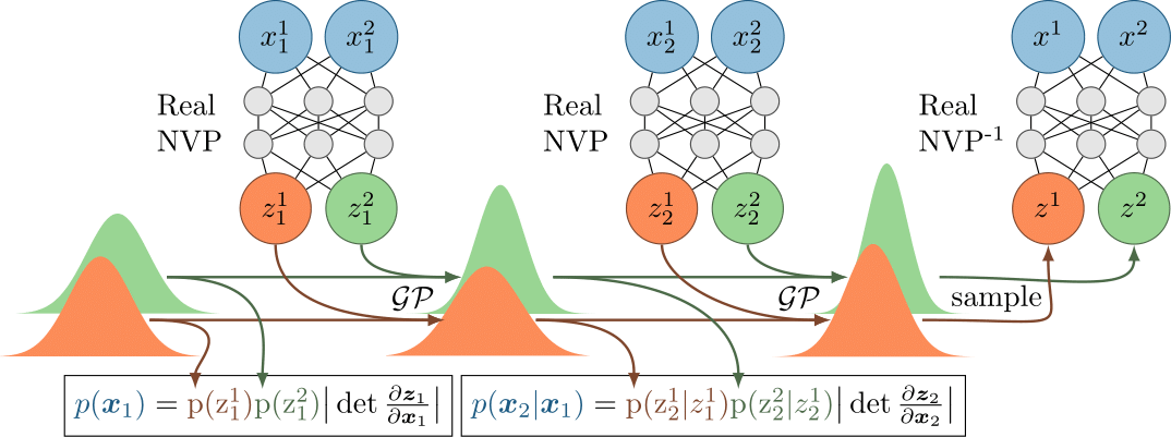
Because we have the predictive probabilities at every step, we can train BRUNO using MLE, where we maximise the likelihood of the inputs with respect to the Real NVP parameters and parameters of GPs kernels: \(\rho\) and \(v\) for every of the \(D\) latent dimensions.

We train BRUNO on a dataset of i.i.d. sequences \(\{(\mathbf x_1, \mathbf x_2, .., \mathbf x_n)_i\}_{i=1..M}\), where we assume that observations within a sequence are exchangeable. This assumption proved reasonable for sequences where observations belong to the same class. In this case, BRUNO should learn some class-specific visual features and also learn that those are correlated across the sequence. It appears to work well for the tasks of few-shot generation and classification, which we will look into next.

Experiments

Omniglot has become a standard dataset for testing few-shot learning algorithms. It is commonly referred to as the “transpose” of MNIST since it has a large number of character classes with only 20 examples per class. So if we train BRUNO on the same-class sequences from Omniglot’s train set, we can easily test its few-shot performance on the unseen characters.

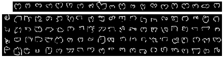
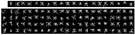
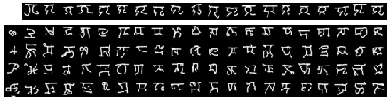
Below are a few examples of generated samples conditionally on an input sequence of unseen characters. The cool thing about BRUNO is that it doesn’t need any retraining on classes it has never seen. We just need to feed BRUNO a test sequence of an arbitrary length and get our n-shot generated images as a result of sampling from a conditional distribution \(p(\mathbf x_{n+1} \mid \mathbf x_{1:n})\).

^{In each subplot, an input sequence is shown in the top row and samples are in the bottom 4 rows. Every column with samples contains 4 samples from the predictive distribution conditioned on the input images up to and including that column. That is, the 1st column shows samples from the prior \(p(\mathbf x)\) when no input image is given; the 2nd column shows samples from \(p(\mathbf x \mid \mathbf x_1)\) where \(\mathbf x_1\) is the 1st input image in the top row and so on.}

---

We can use the very same model for image classification in a n-shot, k-way setup. From the test accuracies below, we see that BRUNO is doing okay, but not as good as Matching Nets. That’s no surprise since BRUNO was trained as a generative model and may have wasted a lot of statistical power on modelling aspects of the data which are irrelevant for the classification task. However, if we now finetune BRUNO with a discriminative objective, i.e. maximising the likelihood of correct labels in few-shot classification episodes, its performance becomes a lot better.

Model	n=1,k=5	n=5,k=5	n=1,k=20	n=5,k=20
Matching Nets	98.1%	98.9%	93.8%	98.5%
BRUNO	86.3%	95.6%	69.2%	87.7%
BRUNO finetuned	97.1%	99.4%	91.3%	97.8%

Another application for BRUNO can be set anomaly detection in a stream of incoming data. To give an example, we trained BRUNO on even MNIST digits and tested on odd digits ³. Below is a plot of how the probabilistic score \(\frac{p(\mathbf x \mid \mathbf x_{1:n})}{p(\mathbf x)}\) evolves when we feed a stream of images into BRUNO, and we see that it picks up the weird looking ones. So if you ever need a low-compute and low-memory app for set anomaly detection that works on inputs it wasn’t trained on, BRUNO might be a way to go.

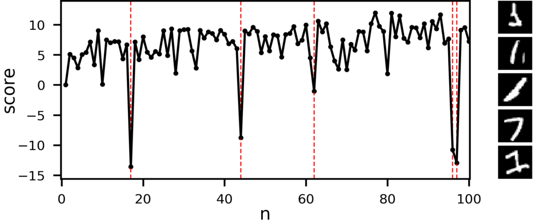
^{Evolution of the score as the model sees more images from a sequence of digit 1 with one image of digit 7. Identified outliers are marked with vertical lines and plotted on the right in the order from top to bottom. Note that the model was trained only on images of even digits.}

---

Conclusion

Exchangeability has recently started gaining more attention in deep learning community and hopefully will go a long way. Some relevant papers include Deep Sets, Neural Statistician and Neural Processes. Compared to them, BRUNO has a bit different flavour: it is an exchangeable process with an intricate analytic form ⁴ defined in the space of high dimensional, complex observations, e.g. images. However, because of a \(\mathcal GP\) + Real NVP construction, this processs is easy to work with and it performs well in practice, so we hope somebody will find it useful.

Code

Our code is available on github: github.com/IraKorshunova/bruno

Notes

---

• ← Previous Post
• Next Post →