The American Epilepsy Society Seizure Prediction Challenge ended a few days ago, and I finished 10th out of 504 teams. In this post I will briefly outline the problem and my solution.
The problem
Epilepsy is one of the most commonly diagnosed neurological disorders. It is characterized by the occurrence of spontaneous seizures, and to make matters even worse nearly 30% of patients cannot control their seizures with medication. In such cases, seizure forecasting systems are vitally important. Their purpose is to trigger a warning when a probability of the forthcoming seizure exceeds a predefined threshold, so patients have time to plan their activities.
As a primary challenge towards building a seizure prediction device is the ability to classify between pre-seizure and non-seizure states of the brain activity measured with the EEG. Further, we will use a term preictal to denote a pre-seizure state and interictal for a normal EEG data without any signs of seizure activity.
Preictal state in our setting was defined to be one hour before the seizure onset with a 5-minute horizon.
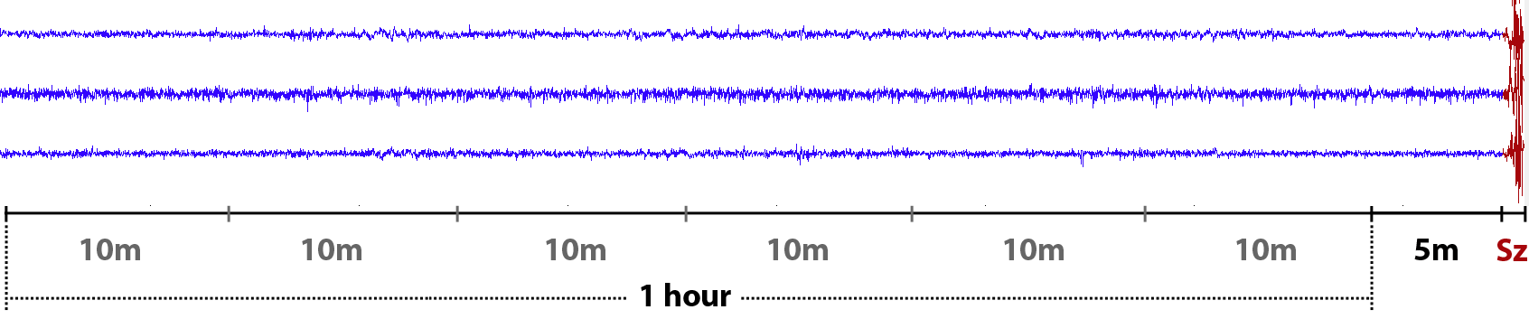
For each 10-minute clip from preictal or interictal one-hour sequence, we were asked to assign a probability that a given clip is preictal. In the training data the timing of each clip was known. However it wasn’t given for the test data clips, so we couldn’t use the timing information when building a classifier.
The evaluation metric was the area under the ROC curve (AUC) calculated for seven available subjects as one big group. It implied an additional challenge since predictions from subject-specific models in general were not well calibrated. Training a single classifier for all subject a priori could not work better because brain activity is a highly individual. The global AUC metric required additional robustness against the choice of the classification threshold, which is crucial in seizure forecasting systems.
The solution: convnets
The idea of using convnets for EEG was inspired by the research of Sander Dieleman. In his case, the audio signal was one-dimensional, unlike the EEG signal, which had 15-24 channels depending on the subject. Therefore, the information from different channels has to be combined in some way. I tried various convnets architectures, however, most success I could get when merging features from different channels in the very first layer.
The input features itself were very simple and similar to those in Howbert et al., 2014: EEG signal was partitioned into nonoverlapping 1 min frames and transformed with DFT. The resulted amplitude spectrum was averaged within 6 frequency bands: delta (0.1-4 Hz), theta (4-8 Hz), alpha (8-12 Hz), beta (12-30 Hz), lowgamma (30-70 Hz) and highgamma (70-180 Hz). Thus, the dimension of the data clip was equal to \(N\times6\times10\) (channels \(\times\) frequency bands \(\times\) time frames). Additionally in some models I used standard deviation of the signal computed in the same time windows as DFT.
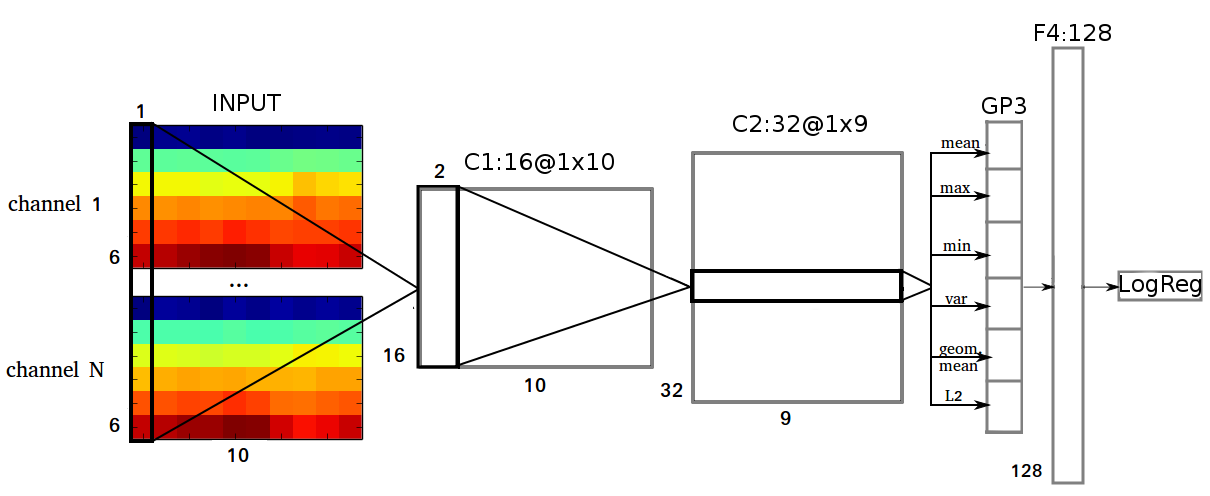
Its first layer (C1) performs convolution in a time dimension over all N channels and all 6 frequency bands, so the shape of its filters is \(6\times N \times 1\). C1 has 16 feature maps each of shape \(1\times10\). The second layer (C2) performs convolution with 32 filters of size \(16\times2\). C2 is followed by a global temporal pooling layer GP3, which computes the following statistics: mean, maximum, minimum, variance, geometrical mean, \(L_2\) norm over 9 values in each feature map from C2. GP3 is fully connected with 128 units in F4 layer. C1 and C2 layers were composed of ReLUs; tanh activation was used in the hidden layer.
I used Python, Theano, NumPy and SciPy to implement the solution. Since I didn’t have a GPU, I trained everything on CPU, which usually took 2-6 hours to train all individual models for 175K gradient updates with ADADELTA.
Model averaging
As a final model I used a geometric mean of the predictions (normalized to 0-1 range for each subject) obtained from 11 convnets with different hyperparameters: number of feature maps or hidden units in each layer, strides in convolutional layers, amount of dropout and weight decay, etc. Models were also trained on different data, for example, I could take DFT in 0.5 or 2 minute windows or change the frequency bands partition by dividing large gamma bands into two. To augment the training set I took the overlaps between consecutive clips in the same one-hour sequence, regretfully I didn’t do it real-time.
Results
In the middle of the competition organizers decided to allow use of the test data to calibrate the predictions. I used the simplest form of calibration: unity-based normalization of per-subject predictions. This could improve the AUC on about 0.01. So the final ensemble, where each of 11 models was calibrated, obtained 0.81087 on public and 0.78354 on private datasets. Models averaging was essential to reduce the probability of an unpleasant surprise on the private LB. After the private scores had become available, I found out that some models with relatively high public scores had unexpectedly low private scores and vice versa. A possible explanation I will give in the next section.
Pitfalls of the EEG
In this competition one could easily overfit to the public test set, which explains a large shake up between public and private leaderboard standings. Moreover, a tricky cross-validation could track the test score with varying success, and simple validation wasn’t even supposed to work. So what is the reason for this phenomena?
The problem lies in the properties of the EEG data: clips, which are close in time are more similar to one another than to the distant clips because brain activity constantly changes. This can be showed via t-SNE. If we take all preprocessed data clips (train and test) from one subject, transform them with PCA into vectors with 50 components and take a few sequences it would look like the plot below. Here we can see three clusters of six 10-minute clips (with some outliers), which correspond to different preictal EEG hours.
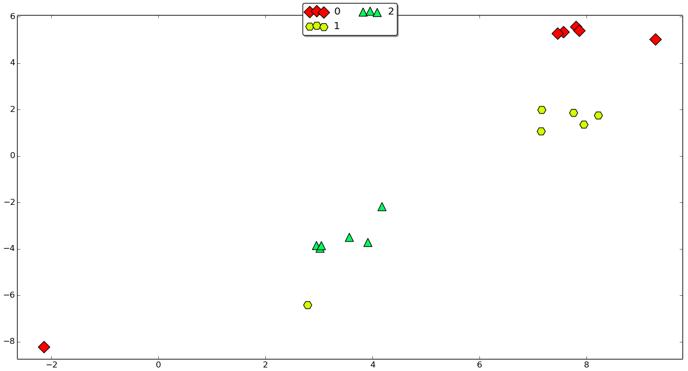
Obviously, if the classifier is trained on 5 clips from a green sequence, it is easier to make a correct predictions for the 6th green clip rather than for yellow or red clip from another sequence. Sadly, but in many papers I’ve seen on seizure prediction, this fact is oftenly neglected. Many authors report cross-validation or validation results, which are unlikely to be as optimistic at test time, when the device is actually implanted in one’s brain.
Conclusions
This competition outlined a lot of open questions in the field of seizure prediction. These problems are solvable, so epilepsy patients hopefully could get reliable seizure advisory systems in the nearest future.
The competition was a basis for my thesis, which can be found in my GitHub repository along with its code.